This page holds supplements to the project When to monitor or control; informed invasive species management using a partially observable Markov decision process (POMDP) framework, in collaboration with Vera Somers, Michael McCarthy and Chris Baker. Refer here to a poster, and a preprint. This work has been published by Methods in Ecology and Evolution, see here. Code accompanying this work is available at this repository.
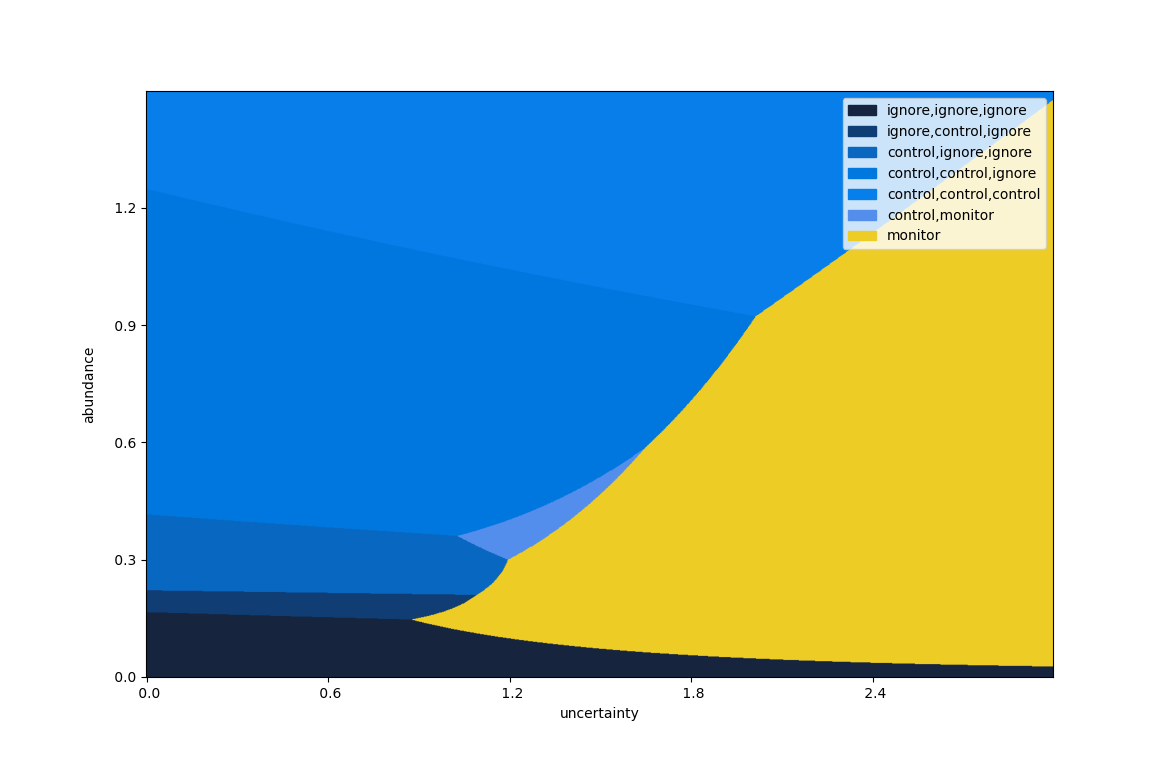
The following is the primary plot from the poster, displaying the optimal management interventions for a theoretical set of parameters (detailed below). A colourblind-friendly version is reproduced also.
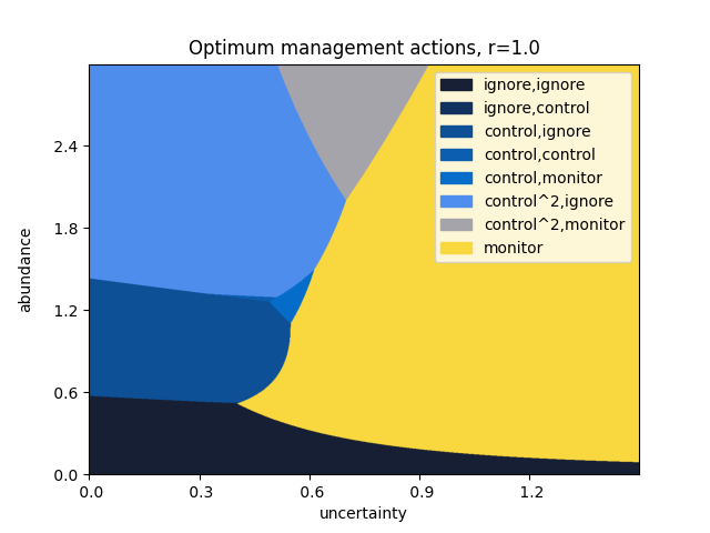
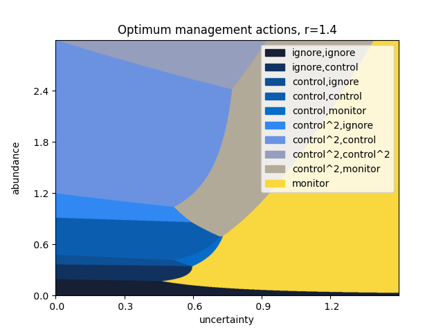
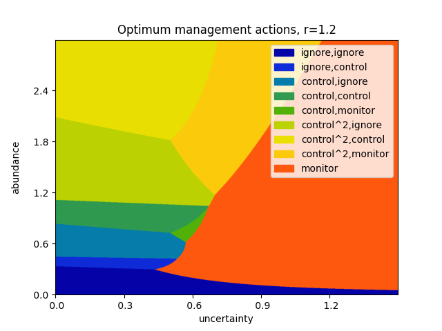
This instance of our model considers three steps in advance, at a discount rate of \(\gamma=0.9\). Monitoring costs \(1\) unit, and has a standard error of \(0.1\). A single control action costs \(4\) units, and reduces the abundance by \(60\%\); correspondingly, controlling twice at once reduces the abundance by \(84\%\) at a cost of \(8\) units. The population is assumed to grow at an exponential rate, with growth parameter \(r = 1.2 \pm 0.05\).
Our model imitates a Belief Space Markov Decision Problem. To deal with the unbounded and continuous state space (species abundance), we limit the form of the managers belief. In the examples we considered, we used a lognormal distribution, so that the state space at time \(t\) is \[ (n_t,\Delta n_t) \in \mathbb{R}\times\mathbb{R}_{\ge 0}. \] Here \(n_t \pm \Delta n_t\) is an estimate of \(\log N\), where \(N = \text{disease abundance}\). For interventions that do not involve monitoring, the transition rule is: \[ n_{t+1} = n_t + r + \log(1-\rho),\quad\text{and}\quad \Delta n_{t+1} = \Delta n_t + \Delta r. \] For monitoring actions, \(n_{t+1}\) is sampled from the distribution defined by \((n_t,\Delta n_t)\), and \(\Delta n_{t+1}\) is determined by a Bayesian update rule. Explicitly: \[ n_{t+1} \sim \text{Norm}(n_t,\Delta n_t^2)\quad \text{and} \quad \Delta n_{t+1} = \frac{\Delta n_t\cdot \text{err}}{\Delta n_t + \text{err}}. \] The cost of each intervention is expressed in units of species abundance, so that the reward at time \(t\) with action \(a_t\) is \[ R_t = \mathbb{E}(N) + \text{cost}(a_t) = \exp(n_t + (\Delta n_t)^2/2) + \text{cost}(a_t). \] With a fixed horizon and discount factor, this MDP can be solved by the usual value iteration techniques.
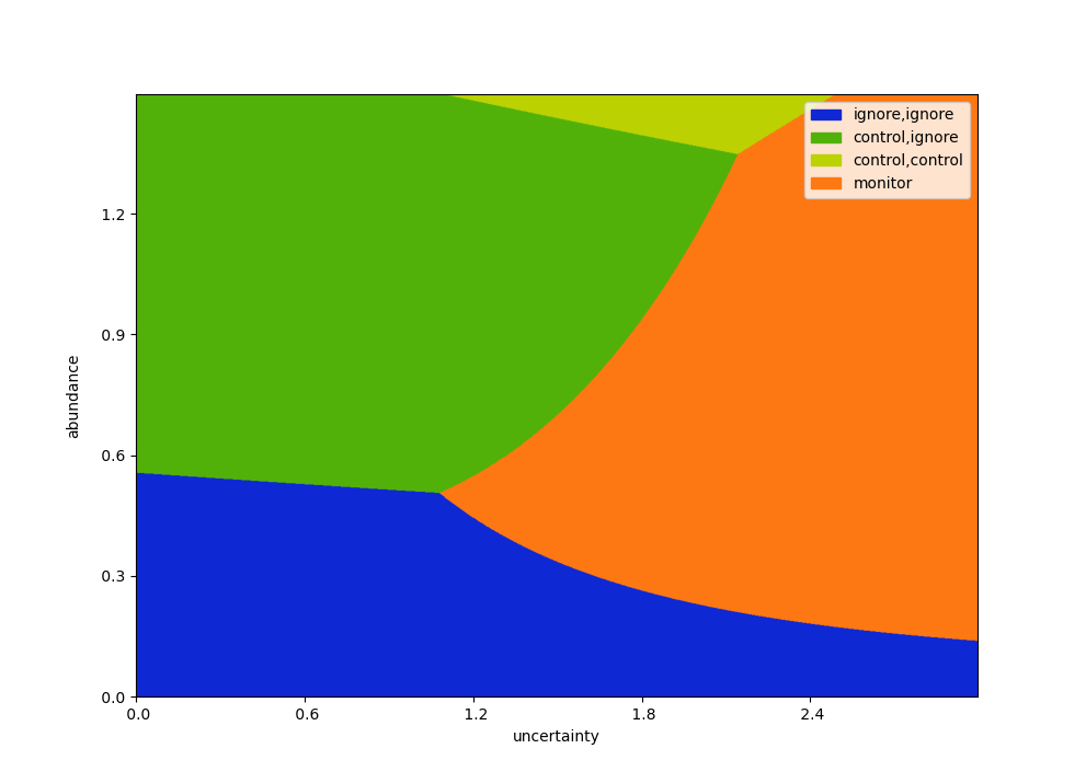
The simplest interesting case is over two steps, with one control and one monitoring intervention, viz:
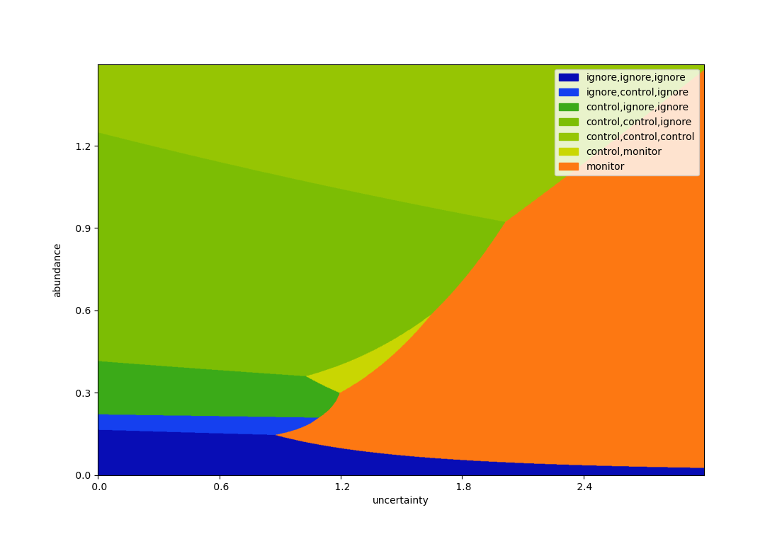
We can extend this is several directions. The plot above consists of adding an extra control intervention (with residual abundance \(1-\rho = (40\%)^2 = 16\%\)), and optimizing with a horizon of three time steps. In our simple case, extending the horizon looks as follows.
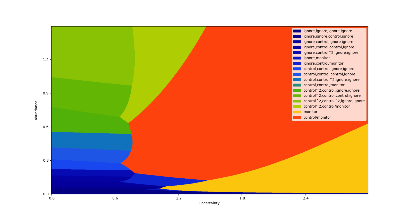
With too many actions and steps, the legend becomes difficult to read, so we display a limited number of steps into the future.
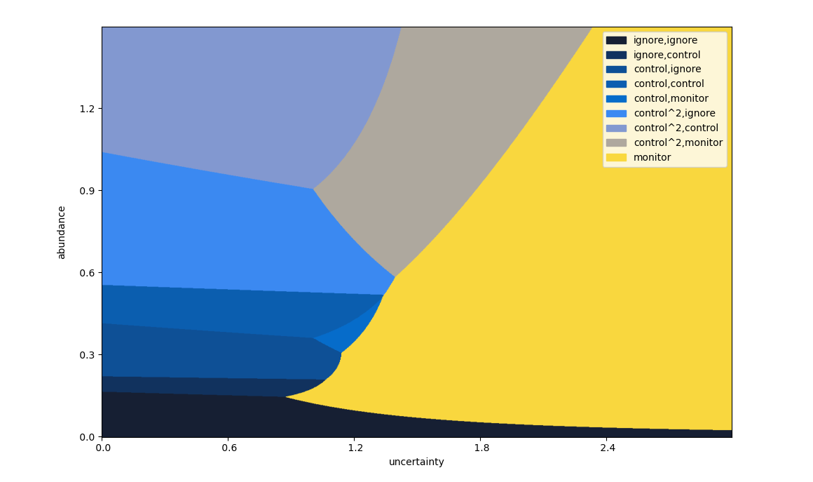
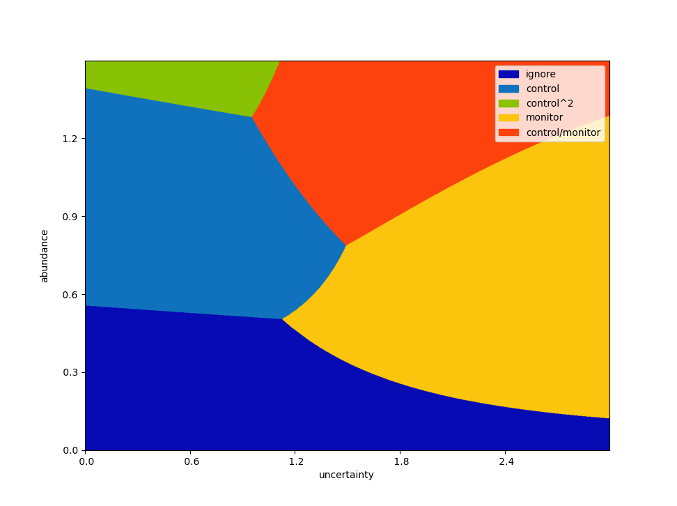
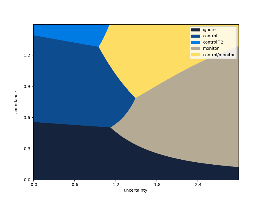
Returning to the two-step case, along with the extra control intervention as above, we can add further monitoring options. For example, the following plot allows for a combined monitoring / control action.
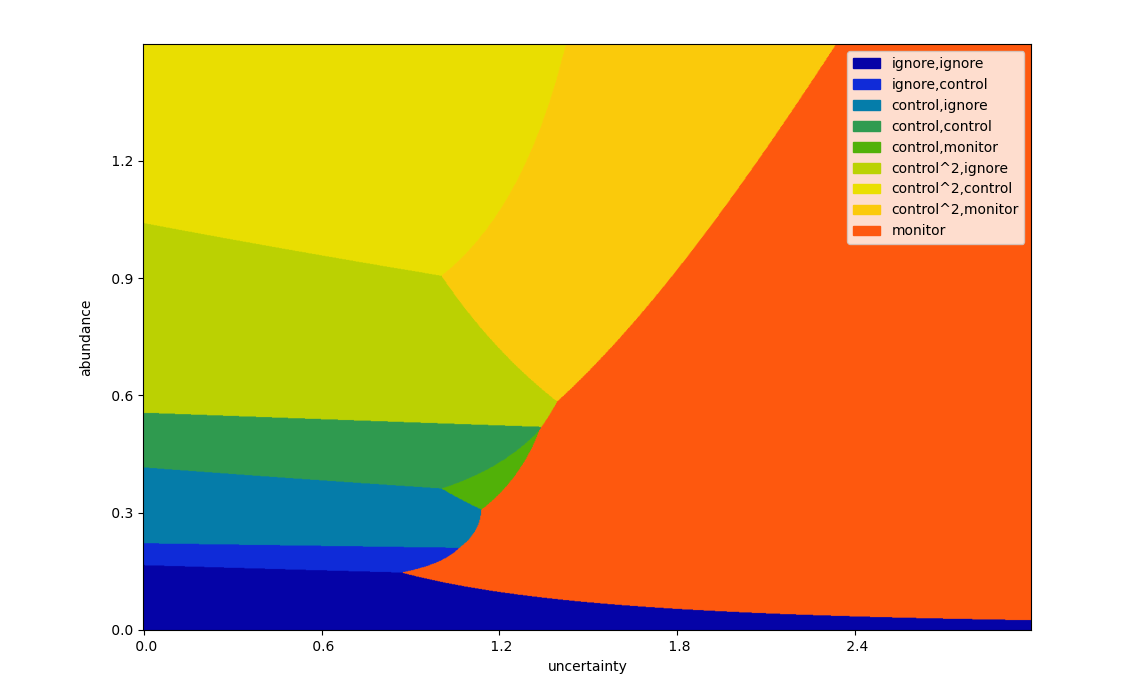
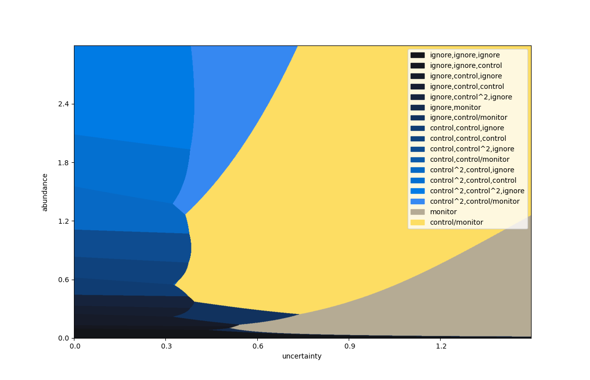
This stretches in any number of directions, including varied effectiveness, costs and monitoring error. As a final example, the following looks four steps into the future, and includes all five options.
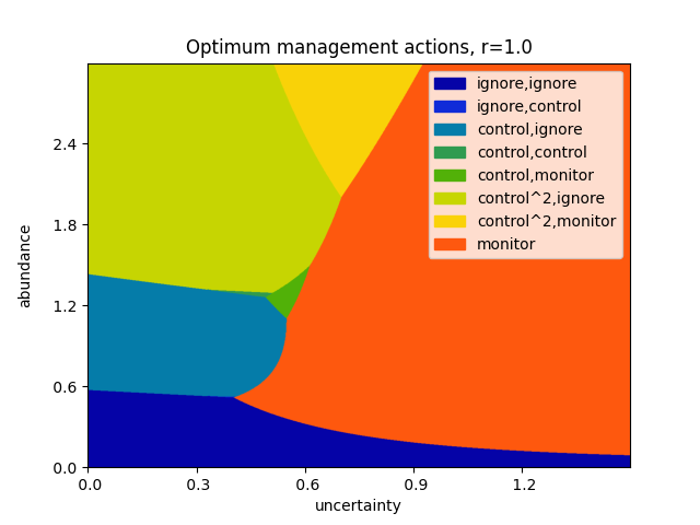
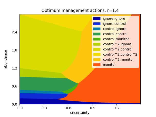
The above plot can be repeated for varying values of the growth rate \(r\).
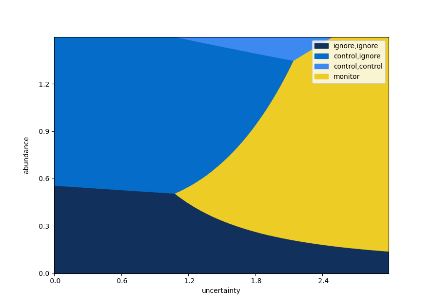
Simple case: two steps, and one control and monitroing option each.
As above, but over three steps.
A two-step plot, with five total options.
A final example, with five options and a longer horizon.
Varying the growth rate, as above.